[1]:
import sisicepy
import sisicepy.traces.traces as st
import sisicepy.traces.io.datacube_loader as stio_dc
import sisicepy.traces.io.mseed_loader as stio_ms
import sisicepy.traces.captor.digos as digos
import numpy as np
import matplotlib.pyplot as plt
import numpy as np
import hvplot.xarray
import pint_xarray
from pint_xarray import unit_registry as ureg

%matplotlib inline
Quick start
This is a quick tutorial to shows how to use sisicepy
Load the data
sisicepy can directly load Digos DataCube file.
adr='/mnt/data2/Planpincieux2024/2-Sismometer/BRG/240611/06120000.BRG'

data=stio_dc.load_datacube(adr,axis=[0,1,2])
It also support mseed:
[2]:
adr='data/c0brg240612000455.pri0'

data=stio_ms.load_mseed(adr,gain=16)
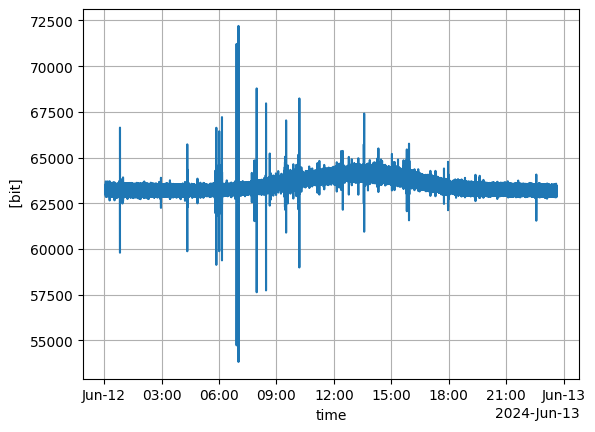
Plot the raw data
[3]:
data.plot()
plt.grid()
Data processing
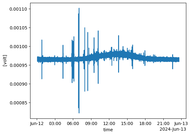
Convert to Volt
Working one one trace
[4]:
tr0=data.traces.count2volt_datacube()
[5]:
tr0.plot()
[5]:
[<matplotlib.lines.Line2D at 0x79adf1511710>]
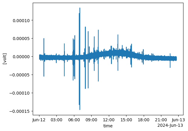
Deconvolution of the signal
Using zeros-poles gains
For digos geophone, the zeros, poles and gains are store in digos.geophone_PZ()function
[6]:
help(digos.geophone_PZ)
Help on function geophone_PZ in module sisicepy.traces.captor.digos:

geophone_PZ()
    Value for Poles and Zeros function of the Digos Geophone

    Zeros: [0,0]
    Poles :[-19.78+20.20i,-19.78-20.20i]
    K=27.7 V/(m.s^-1)
Therefore it can be apply afer removing the mean and the trend:
[7]:
tr0_clean=tr0.traces.remove_mean().traces.remove_trend()
/home/chauvet/miniforge3/envs/sisicepy/lib/python3.11/site-packages/xarray/core/variable.py:341: UnitStrippedWarning: The unit of the quantity is stripped when downcasting to ndarray.
  data = np.asarray(data)
[8]:
tr0_clean.plot()
[8]:
[<matplotlib.lines.Line2D at 0x79ad65185ed0>]
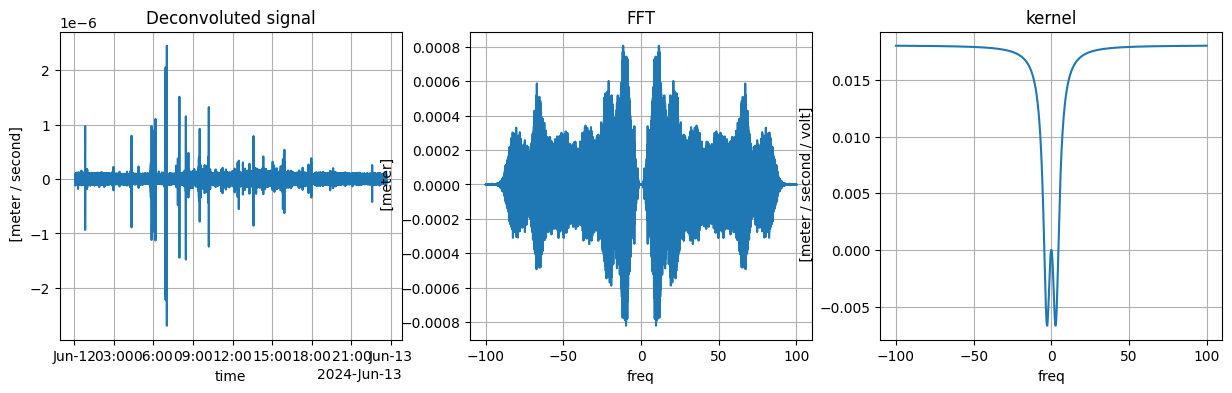
[18]:
signal_deconv,fft_deconv,kernel_deconv=tr0_clean.traces.poles_zeros_filter(digos.geophone_PZ(),10**0)
/home/chauvet/miniforge3/envs/sisicepy/lib/python3.11/site-packages/xarray/core/variable.py:341: UnitStrippedWarning: The unit of the quantity is stripped when downcasting to ndarray.
  data = np.asarray(data)
[19]:
plt.figure(figsize=(15,4))
plt.subplot(131)
signal_deconv.plot()
plt.title('Deconvoluted signal')
plt.grid()
plt.subplot(132)
fft_deconv.real.plot()
plt.title('FFT')
plt.grid()
plt.subplot(133)
kernel_deconv.real.plot()
plt.title('kernel')
plt.grid()
Band filter
Band filter using trapez shape
[11]:
help(st.trapezoid)
Help on function trapezoid in module sisicepy.traces.signal.freq_filter:

trapezoid(self, band, delta)
    Trapeziod band filter:
    .. line-block::
        ........Lower band...........Higher band........
        ........band[0]...............band[1]...........
        ...........|------------------|.................
        ..........||..................||................
        .........|||..................|||...............
        ........||||..................||||..............
        .......|||||..................|||||.............
        ......||||||..................||||||............
        _____|||||||..................|||||||_______....
        .......delta..................delta.............


    :param self: signal to filter with trapeziode band
    :type self: xr.DataArray
    :param band: lower band and higher band ex: [4.5,90] Hz
    :type band: list
    :param delta: delta for the begining and the end of the trapez
    :type delta: float
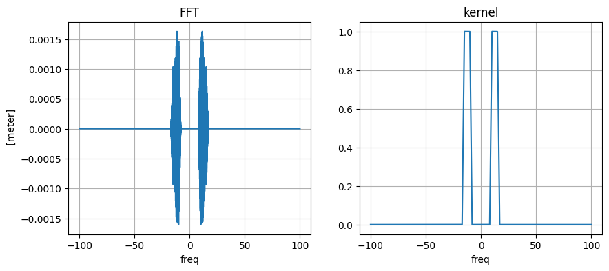
Between 10 and 15 Hz
[12]:
band = [10,15] # Hz
delta = 2 # Hz

signal_deconv_10_15,fft_deconv_10_15,kernel_deconv_10_15=signal_deconv.traces.trapezoid(band,delta)
/home/chauvet/miniforge3/envs/sisicepy/lib/python3.11/site-packages/xarray/core/variable.py:341: UnitStrippedWarning: The unit of the quantity is stripped when downcasting to ndarray.
  data = np.asarray(data)
[13]:
plt.figure(figsize=(10,4))
plt.subplot(121)
fft_deconv_10_15.real.plot()
plt.title('FFT')
plt.grid()
plt.subplot(122)
kernel_deconv_10_15.real.plot()
plt.title('kernel')
plt.grid()
[14]:
di="2024-06-12T04:00:00"
df="2024-06-12T04:00:10"

plt.figure(figsize=(15,6))
signal_deconv_10_15.sel(time=slice(di, df)).plot()
[14]:
[<matplotlib.lines.Line2D at 0x79ad594cf210>]

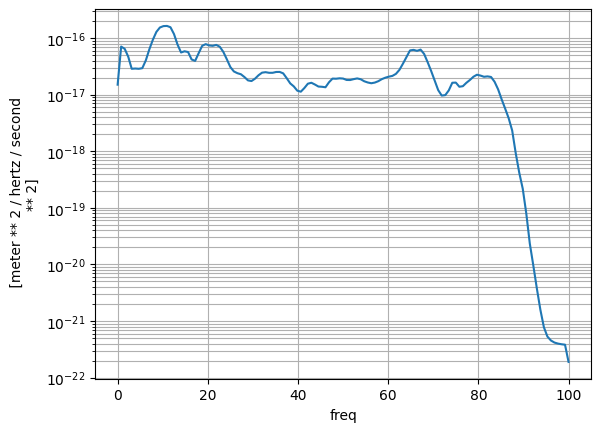
Power Spectral Density
[15]:
signal_PSD=signal_deconv.traces.PSD()
/home/chauvet/miniforge3/envs/sisicepy/lib/python3.11/site-packages/xarray/core/variable.py:341: UnitStrippedWarning: The unit of the quantity is stripped when downcasting to ndarray.
  data = np.asarray(data)
[16]:
signal_PSD.plot(yscale='log')
plt.grid(True, which="both")
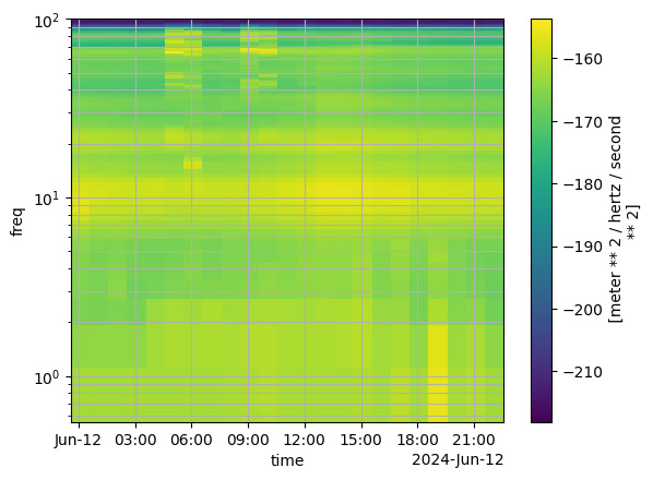
Spectrogram
[17]:
di="2024-06-12T00:00:00"
da_spec=signal_deconv.traces.spectrogram(3600,di,dB=True)
da_spec[1::,:].plot(yscale='log')
plt.grid(True, which="both")
/home/chauvet/miniforge3/envs/sisicepy/lib/python3.11/site-packages/xarray/core/variable.py:341: UnitStrippedWarning: The unit of the quantity is stripped when downcasting to ndarray.
  data = np.asarray(data)